data.table

A basic overview and comparison to common tidyverse functions

By: Nick Garner for UQRUG

What is data.table and why use it?

• It’s the high performance version of base R’s data.frame for manipulation
  • Very fast
  • Memory efficient
  • Lots of features similar to dplyr and other tidyverse functions
  • Great support and documentation + no other dependencies
• Downsides?
  • Can be complex to learn
  • Less intuitive than the tidyverse
  • Less niche features compared to the tidyverse (ie. The complete() function)
  • Isn’t a complete ‘verse’ – ie. No plotting

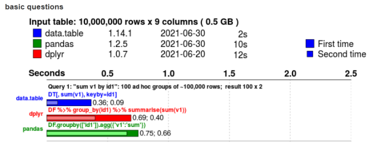
How fast is it?

500MB

5GB

50GB

What can it do?

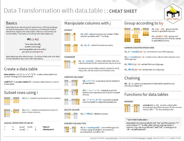
Most of the functions of dplyr and a bit more:

• Manipulate

• Filter

• Sort

• Compute

• Group by

• Bind rows / columns

• Joining columns

• Wide – Long format

• Read + Write files

Almost everything you’d need to reshape data

Loading in and writing out data

• Base/ Tidyverse R: read.csv() or read.xls() -> Becomes a data frame
  • Works well and has a viewer for easy column determination
  • Can change to a data.table by setDT () or as.data.table ()
  • Similar write.csv() etc. to write it to a file.

• data.table: fread () -> Straight into a data.table format
  • Functions identically to a data.frame
  • Very fast to read in data and doesn’t load it all onto RAM (lazy loading)
  • Can read zipped and compressed files without saving a decompressed file
  • Use fwrite () to also write out data much faster (I’ve come across issues here)

Syntax (The hard part!)

tidyverse

Ethos: Do one thing at a time

Each function has an easy to understand name

Example:

Ex2 <- Example %>%

filter(Fruit == "Apples") %>%

group_by*(Variety) %>%

summarise(Weight.mean = mean(Weight))

data.table

Ethos: Do all functions similarly and concisely

Example:

Ex2 <- Example[Fruit == "Apples",
                Weight.mean := mean(Weight)),
                by = "Variety"]

Will run substantially faster on a big dataset

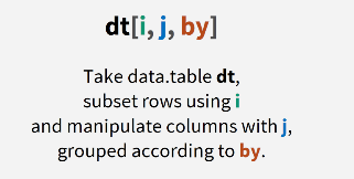
The basic data.table syntax

Example dataset:

Fruit	Variety	Weight
Orange	Navel	400
Apple	Jazz	300
Apple	Jazz	400
…	…	…

Filter a row:

Example[Fruit == "Orange"]

Filter and add a row:

Example[Fruit == "Apple", Fruit_Variety := paste(Variety,Fruit)]

Just add a row:

Example[,BaseCost := (Weight/1000) * 2]

Perform a grouped summary

Example[, by = "Fruit", Fruit_Weight := mean(Weight)]

Moving from the tidyverse to data.table

• Calling a data.table or data.frame: The same (almost)
  • In the tidyverse you can call the df within the function ie. select( df _ , …) _ or before df _ %>% select()_ . In data.table it’s only df[…]
• Manipulating data:
  • In the tidyverse you just use = , ie. mutate( df , ColB _ = _ ColA _ * 10)_
  • In data.table you use := or .() , ie. df [,.( ColB _ = _ ColA _ * 10 )] _ or _ _ df [,:= …]
  • Important to note above df [, … ] not df […] because this tries to subset (filter)
• Chaining functions:
  • In the tidyverse you use the pipe %>%
  • In data.table you can use %>% but better to use dt specific chaining df […][…][…]
  • Using %>% looks like df […] %>% .[…] %>% .[…]

Chaining in data.table

Why Chain? Lots of concise alterations, and less objects saved

• data.table specific chaining looks like df […][…][…]

“I want to know all the types of fruit that will cost on average above $1 per item in order of most to least expensive”

Example2 <- Example[, Fruit_Weight := mean(Weight), by = "Fruit"][, ItemCost := (Weight/1000) * Cost.kg][ItemCost >= 1]\[order(Item)]

• Note: mutate( df , A = 1, B = A + 2) is not the same as df [,.(A = 1, B = A + 2)]

Tidyverse

Example2 <- Example %>%
group_by(Fruit) %>%
summarise(Fruit_Weight = mean(Weight))  %>%
Ungroup() %>%
Mutate(ItemCost = (Weight/1000) * Cost.kg)  %>%
Filter (ItemCost >= 1)  %>%
Arrange(Item)

data.table with pipes

Example2 <- Example[,Fruit_Weight := mean(Weight), by = "Fruit"] %>%
.[,ItemCost := (Weight/1000) * Cost.kg] %>%
.[ItemCost >= 1] %>%
.[order(Item)] 

Example dataset:

Fruit	Variety	Weight	Cost.kg
Orange	Navel	400	2
Apple	Jazz	300	4
Apple	Gala	400	4.5
…	…	…

Some similar functions:

1. filter() ,mutate(), group_by ()

2. summarise(df, sum(ColA), sd (ColB))

3. arrange(df, ColA)

4. select(df, ColA, ColB, ColD)

5. group_by(df, ColA)

6. gather()

7. spread()

8. full_join()

1. Intrinsic df[ filter, mutate, by = ]

2. df[,.(sum = ColA, sd(ColB))]

3. df[order(ColA)]

4. df[,.(ColA, ColB, ColD)]

5. df[,by = ColA] or df[,keyby = ColA]

6. melt()

7. dcast()

8. merge(all = “true”)

The lazy way – improve your code sooner

You: *“I really want to use _ data.table* _ to speed things up but I don’t have time to learn it or alter my pre-existing code”

Me: Give dtplyr a try?

dtplyr allows you to write dplyr code that is automatically translated to the equivalent data.table code under the hood.

Just load the package library( dtplyr ) and use df2 <- lazy_dt ( df ) before performing your normal operations. At the end use as.data.table () or as_tibble ()

Final notes

• Some code doesn’t translate well between the two – Try to check on your data frames often especially when you start using this

• Be careful with ordering, grouping, and manipulating or joining.

  • The speed of data.table can deceive you into thinking you performed a simple normal mutation instead of creating 100x more rows with duplications everywhere

• Running some package functions within data.table that don’t run efficiently won’t be much faster. Ie. The package creator wrote the code using tidyverse dependencies

Extra Resources:

Package information page:

https://rdatatable.gitlab.io/data.table/

Github wiki:

https://github.com/Rdatatable/data.table/wiki/Getting-started

A great comparison website between data.table and dplyr (I use this a lot):

https://atrebas.github.io/post/2019-03-03-datatable-dplyr/