'data.frame':   32 obs. of  11 variables:
 $ mpg : num  21 21 22.8 21.4 18.7 18.1 14.3 24.4 22.8 19.2 ...
 $ cyl : num  6 6 4 6 8 6 8 4 4 6 ...
 $ disp: num  160 160 108 258 360 ...
 $ hp  : num  110 110 93 110 175 105 245 62 95 123 ...
 $ drat: num  3.9 3.9 3.85 3.08 3.15 2.76 3.21 3.69 3.92 3.92 ...
 $ wt  : num  2.62 2.88 2.32 3.21 3.44 ...
 $ qsec: num  16.5 17 18.6 19.4 17 ...
 $ vs  : num  0 0 1 1 0 1 0 1 1 1 ...
 $ am  : num  1 1 1 0 0 0 0 0 0 0 ...
 $ gear: num  4 4 4 3 3 3 3 4 4 4 ...
$ carb: num 4 4 1 1 2 1 4 2 2 4 ...Basic Statistics
Basic Statistics
This is simply a presentational form of the code shown during the August UQRUG.
Load the libraries and data
Explore the data structure
Descriptive statistics
The summary() function provides quick and easy descriptive statistics, and is useful initial step:
      mpg             cyl             disp             hp
 Min.   :10.40   Min.   :4.000   Min.   : 71.1   Min.   : 52.0
 1st Qu.:15.43   1st Qu.:4.000   1st Qu.:120.8   1st Qu.: 96.5
 Median :19.20   Median :6.000   Median :196.3   Median :123.0
 Mean   :20.09   Mean   :6.188   Mean   :230.7   Mean   :146.7
 3rd Qu.:22.80   3rd Qu.:8.000   3rd Qu.:326.0   3rd Qu.:180.0
 Max.   :33.90   Max.   :8.000   Max.   :472.0   Max.   :335.0
      drat             wt             qsec             vs
 Min.   :2.760   Min.   :1.513   Min.   :14.50   Min.   :0.0000
 1st Qu.:3.080   1st Qu.:2.581   1st Qu.:16.89   1st Qu.:0.0000
 Median :3.695   Median :3.325   Median :17.71   Median :0.0000
 Mean   :3.597   Mean   :3.217   Mean   :17.85   Mean   :0.4375
 3rd Qu.:3.920   3rd Qu.:3.610   3rd Qu.:18.90   3rd Qu.:1.0000
 Max.   :4.930   Max.   :5.424   Max.   :22.90   Max.   :1.0000
       am              gear            carb
 Min.   :0.0000   Min.   :3.000   Min.   :1.000
 1st Qu.:0.0000   1st Qu.:3.000   1st Qu.:2.000
 Median :0.0000   Median :4.000   Median :2.000
 Mean   :0.4062   Mean   :3.688   Mean   :2.812
 3rd Qu.:1.0000   3rd Qu.:4.000   3rd Qu.:4.000
 Max.   :1.0000   Max.   :5.000   Max.   :8.000
Visualise the data
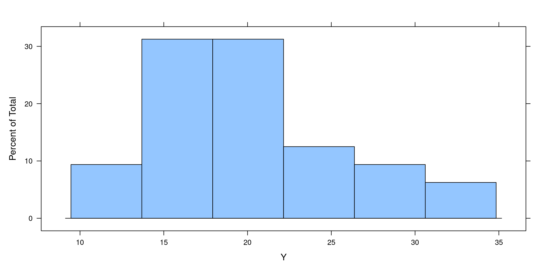
With histogram() we can quickly view the descriptive stats plots per variable

Visualise the data
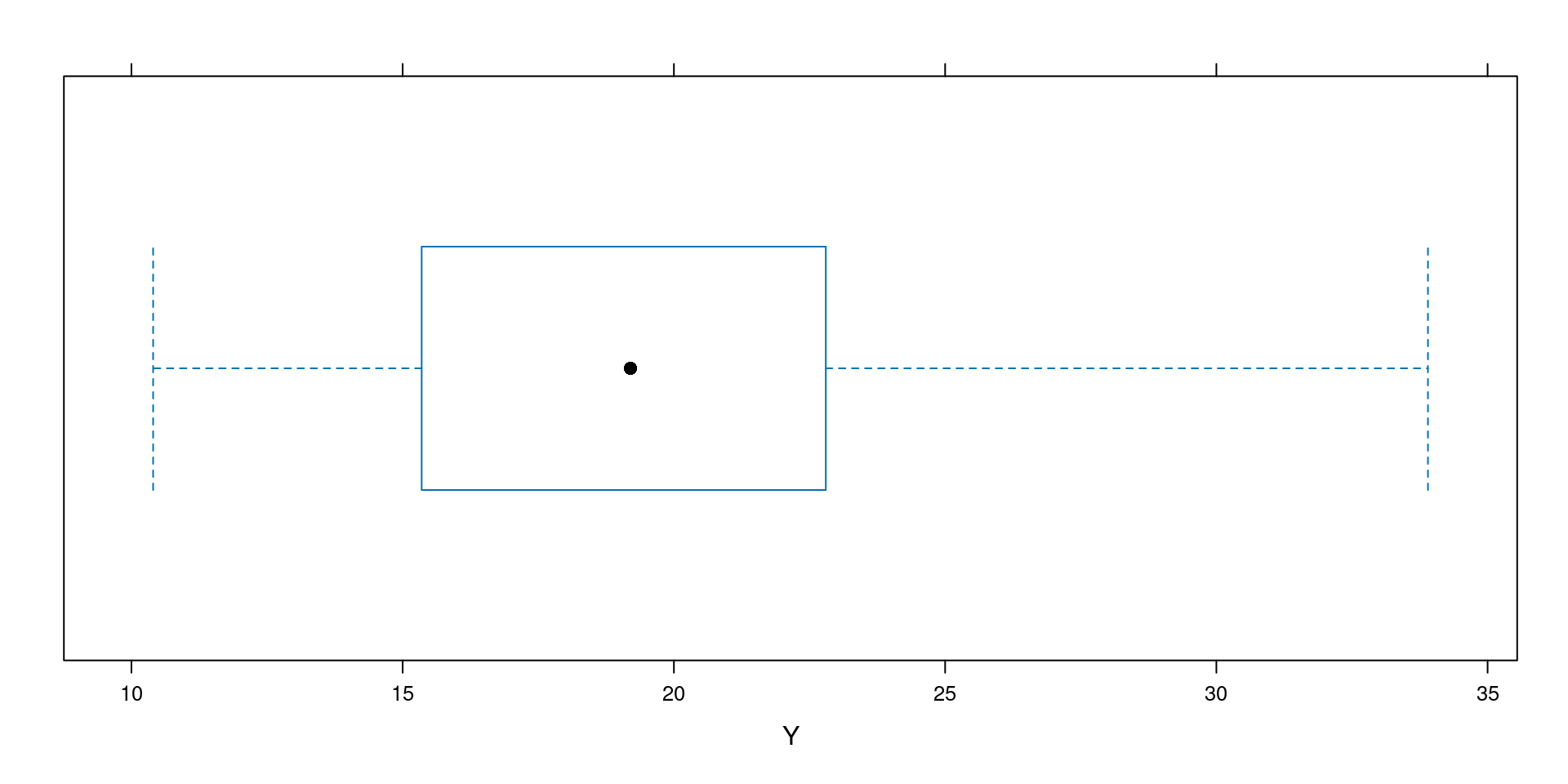
Box and whisker plots are another useful way to visualise our data spread quickly and easily with bwplot()

Inferential statistics
The classic two sample t-test can easily be run with the t.test() function
    Welch Two Sample t-test

data:  time by daytime
t = -6.8311, df = 77.776, p-value = 1.667e-09
alternative hypothesis: true difference in means between group 1 and group 2 is not equal to 0
95 percent confidence interval:
 -48.78467 -26.76533
sample estimates:
mean in group 1 mean in group 2
        967.900        1005.675
ANOVA visualisation
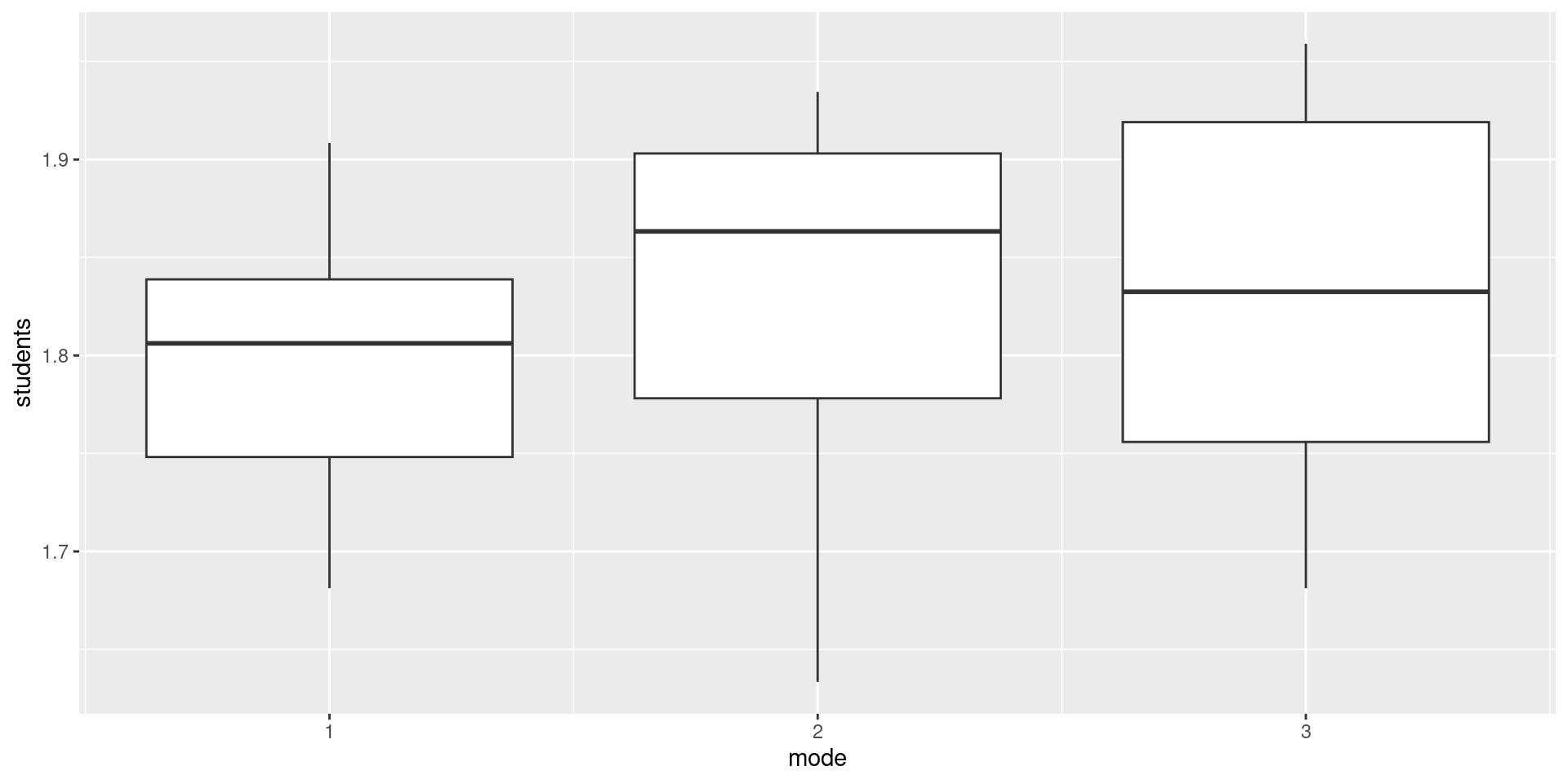
Before we run the ANOVA test, it can be a good idea to visualise our data with a boxplot, which ggplot2 also has

ANOVA
An ANOVA is a good test to determine if the means of multiple independent variables are equal
            Df Sum Sq  Mean Sq F value Pr(>F)
mode         1 0.0191 0.019093   2.953 0.0889 .
Residuals   97 0.6272 0.006466
---
Signif. codes:  0 '***' 0.001 '**' 0.01 '*' 0.05 '.' 0.1 ' ' 1
Correlation
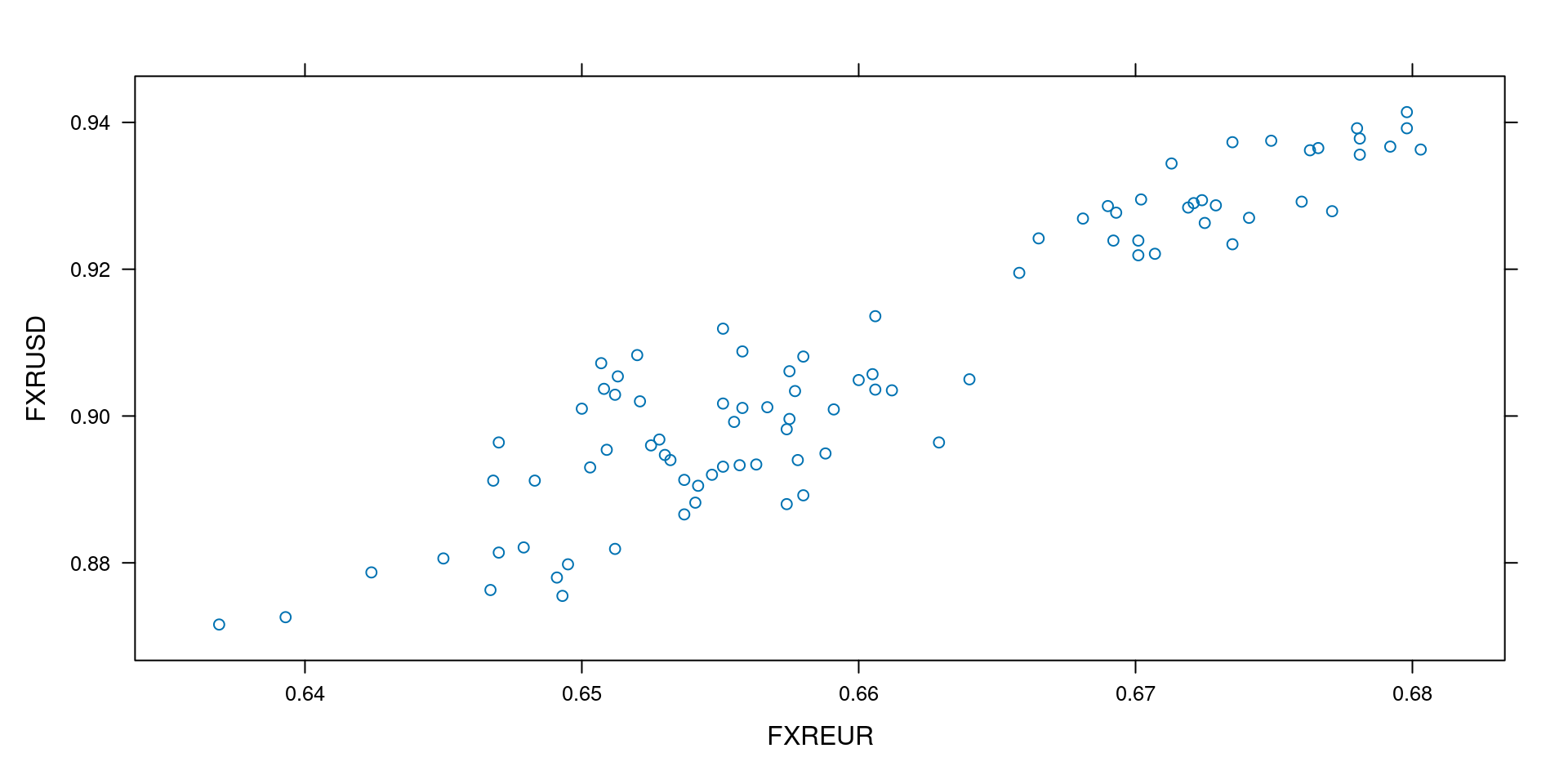
Before running a corrlelation test, it is good to visualise the relationship of the data with a simple scatterplot such as the lattice xyplot()

Correlation
We can now test for correlation using a Pearson or Spearman test
[1] 0.933557[1] 0.872435Linear Regression
Call:
lm(formula = FXRUSD ~ FXREUR, data = data4)

Coefficients:
(Intercept)       FXREUR
     -0.190        1.662